EbayesThresh Toy ex

ITSTGCN

Author

SEOYEON CHOI

Published

July 18, 2023

Import

from itstgcn.learners import *

import numpy as np
import matplotlib.pyplot as plt
import random
import pandas as pd

from rpy2.robjects.vectors import FloatVector
import rpy2.robjects as robjects
from rpy2.robjects.packages import importr
import rpy2.robjects.numpy2ri as rpyn
ebayesthresh = importr('EbayesThresh').ebayesthresh

While \({\bf p}_y\) serves as a consistent estimator for \(\mathbb{E}[|{\bf V}^H{\bf y}|^2]\), it is not an efficient estimator, and therefore, improvement is needed [@djuric2018cooperative]. The traditional approach for improvement is to use the windowed periodogram.
The windowed periodogram is efficient in detecting specific frequencies or periods, but it may not be as efficient in estimating the underlying function. One notable paper that utilized the windowed periodogram is the one that detected the El Niño phenomenon.
As this structure exhibits a “sparse signal + heavy-tailed” characteristics, by applying Bayesian modeling and thresholding \({\bf p}_y\), we can estimate an appropriate \({\bf p}_{pp}\) as discussed in [@johnstone2004needles].

Bayesian Model

\(x_i \sim N(\mu_i,1)\)

확률변수가 잘 정의되어 있을때, 여기서 \(\mu_i\)를 정하는 Baysian.

\(\mu_i \sim\) 사전분포(\(\mu_i\)를 뽑을 수 있는)
\((\mu_i | X_i = x_i)^n_{i=1} \sim\) 사후분포

ex) \(N(10,1) \sim\) 사전분포

관측치

_obs = [7.1,6.9,8.5]

np.mean(_obs)

7.5

관측치를 보니 평균이 10이 아닌 것 같다.

\(N(10-3,1) \sim\) 사후분포

여기서, \(10-3\)이 posterior meman
사후 분포를 정의할때, 이벤트의 mean이냐, median이냐로 잡는 방법은 정해진 것이 아니다.(이베이즈에서는 median으로 잡음)

Ebayes는 사전분포를 Heavy-tail으로 정의했다.

heavy tail?

\(\mu_x \sim\) Double Exponential \(= p_{pp} + p_{ac}\) -> 혼합형(misture) = pure point + absolutely continuous

\(E(\mu_i | X_i = x_i) = \hat{\mu}_i\) -> thresholding의 결과

\(f_{prior}(\mu) = (1-w)\delta_0(\mu) + w \gamma (\mu)\)

\(\delta_0\) = 디렉함수(특정값이 아니면 다 0으로 봄)
\(\gamma = \frac{a}{2} e^{-a|\mu|}\)

Ebayes의 역할 = 자동으로 \(w\)를 계산 혹은 추정

\(1-w\) 확률로 \(\delta_0\)를 정의, \(w\)의 확룔로 \(\gamma\)를 정의.

\(X_i = \mu_i + \epsilon_i, \epsilon_i \sim N(0,1)\)에서 \(\mu_i\)를 찾는게 목적이다. 이게 바로 \(\eta\)값

Ebayes로 sparse signal만 골러낼 것이다.
평균 이상의 값에서 자를 것이다.
- thresh(임계치)를 잡는 게 어려울 텐데, 위에서 이베이즈가 \(w\)를 자동으로 잡아 확률 계산되는 방법론을 제안한 것,
baysian modeling 사용하여 heavy tail + impulse(sparse)에서 posterior median 추정하여 임계값thresh으로 \(p\)에서 \(p_{pp}\)를 추출하는 것이 GODE 목적

EbayesThresh

T = 100

t = np.arange(T)/T * 10

y_true = 3*np.sin(0.5*t) + 1.2*np.sin(1.0*t) + 0.5*np.sin(1.2*t)

y = y_true + np.random.normal(size=T)

plt.figure(figsize=(10,6))
plt.plot(t,y_true)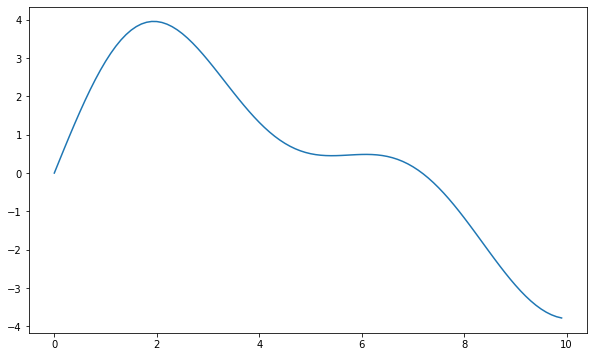

- 관찰한 신호

plt.plot(t,y,'o')
plt.plot(t,y_true,'--')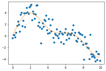

- 퓨리에 변환

f = np.array(y)
if len(f.shape)==1: f = f.reshape(-1,1)
T,N = f.shape
Psi = make_Psi(T)
fbar = Psi.T @ f # apply dft

plt.plot(t,fbar**2) # periodogram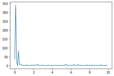

- threshed

fbar_threshed = np.stack([ebayesthresh(FloatVector(fbar[:,i])) for i in range(N)],axis=1)
plt.plot((fbar**2)) # periodogram 
plt.plot((fbar_threshed**2))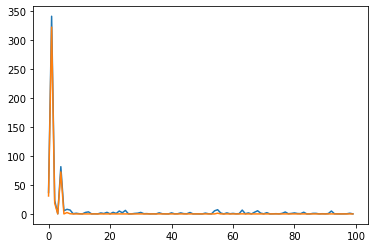

plt.plot((fbar**2)[20:80]) # periodogram 
plt.plot((fbar_threshed**2)[20:80])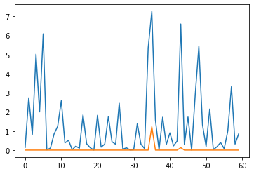

- 역퓨리에변환

yhat = Psi @ fbar_threshed # inverse dft

plt.figure(figsize=(10,6))
plt.plot(t,y,'.')
plt.plot(t,y_true,'--')
plt.plot(t,yhat)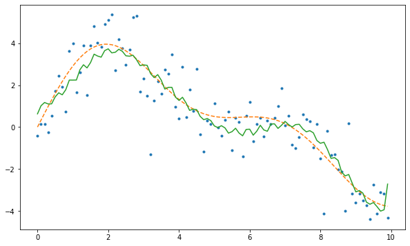

plt.figure(figsize=(10,6))
plt.plot(y,'.')
plt.plot(y_true)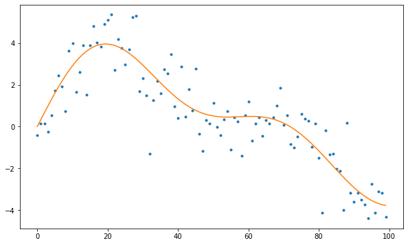

Result

with plt.style.context('seaborn-white'):
    fig, ((ax1,ax2),(ax3,ax4)) = plt.subplots(2,2,figsize=(40,15))
    fig.suptitle('Figure 1',fontsize=40)
    
    ax1.plot(y, 'b.',alpha=0.5)
    ax1.plot(y_true,'p--',label='True')
    ax1.legend(fontsize=20,loc='upper left',facecolor='white', frameon=True)
    
    ax1.tick_params(axis='y', labelsize=20)
    ax1.tick_params(axis='x', labelsize=20)
    
    ax2.plot(y, 'b.',alpha=0.5)
    ax2.plot(y_true,'p--',label='True')
    ax2.plot(yhat,label='y hat')
    ax2.legend(fontsize=20,loc='upper left',facecolor='white', frameon=True)
    ax2.tick_params(axis='y', labelsize=20)
    ax2.tick_params(axis='x', labelsize=20)
    
    ax3.plot((fbar**2)) # periodogram 
    ax3.plot((fbar_threshed**2)) 
    ax3.tick_params(axis='y', labelsize=20)
    ax3.tick_params(axis='x', labelsize=20)
    ax3.axvspan(20, 80, facecolor='gray', alpha=0.2)

    
    ax4.plot(range(20, 80),(fbar**2)[20:80]) # periodogram 
    ax4.plot(range(20, 80),(fbar_threshed**2)[20:80]) 
    ax4.set_xticks(range(20, 81, 10))
    ax4.set_xticklabels(range(20, 81, 10))
    # ax4.set_xticklabels(['20','40','60'])
    ax4.tick_params(axis='y', labelsize=20)
    ax4.tick_params(axis='x', labelsize=20)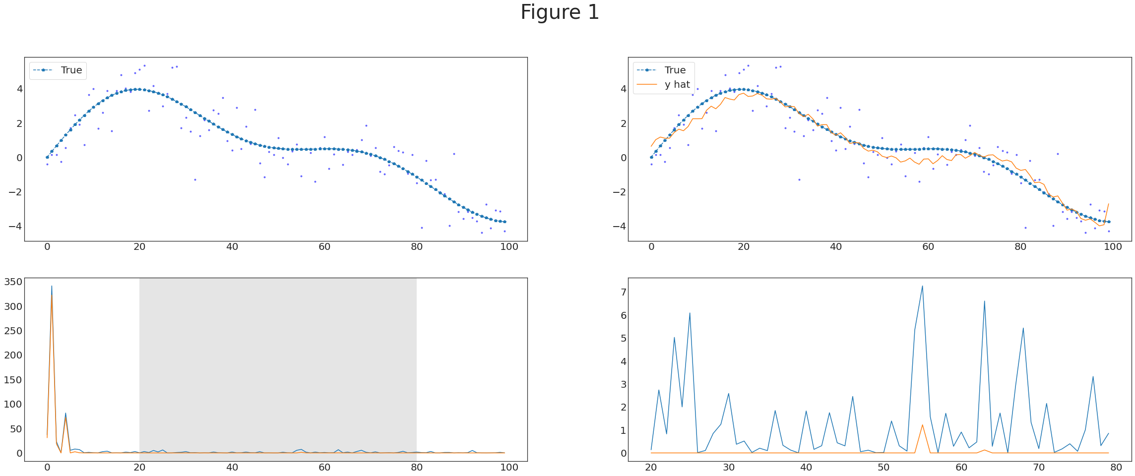

from mpl_toolkits.axes_grid1.inset_locator import mark_inset, inset_axes
plt.figure(figsize = (20,10))
plt.suptitle('Figure',fontsize=40)
ax = plt.subplot(1, 1, 1)
ax.plot(range(0,100),(fbar**2))
ax.plot((fbar_threshed**2)) 
axins = inset_axes(ax, 8, 3, loc = 1, bbox_to_anchor=(0.8, 0.8),
                   bbox_transform = ax.figure.transFigure)
axins.plot(range(20, 80),(fbar**2)[20:80])
axins.plot(range(20, 80),(fbar_threshed**2)[20:80]) 
axins.set_xlim(20, 80)
axins.set_ylim(-0.1, 7)
mark_inset(ax, axins, loc1=4, loc2=3, fc="none", ec = "0.01")
ax.tick_params(axis='y', labelsize=20)
ax.tick_params(axis='x', labelsize=20)
axins.tick_params(axis='y', labelsize=15)
axins.tick_params(axis='x', labelsize=15)
# plt.savefig('Ebayes_Toy.png')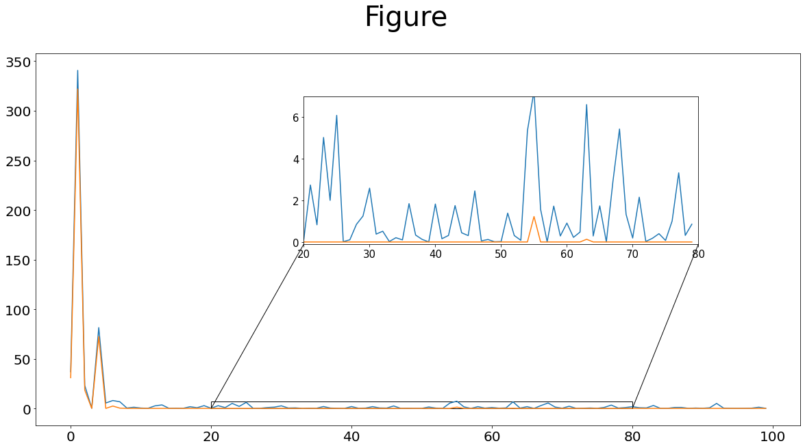

from matplotlib.patches import ConnectionPatch
fig = plt.figure(figsize=(20,10))
plt.suptitle('Figure 1',fontsize=40)
plot1 = fig.add_subplot(2,2,(1,2))

plot1.plot(range(20, 80),(fbar**2)[20:80]) # periodogram 
plot1.plot(range(20, 80),(fbar_threshed**2)[20:80]) 
plot1.set_xticks(range(20, 81, 10))
plot1.set_xticklabels(range(20, 81, 10))
plot1.tick_params(axis='y', labelsize=20)
plot1.tick_params(axis='x', labelsize=20)

plot3 = fig.add_subplot(2,2,(3,4)) 

plot3.plot((fbar**2)) # periodogram 
plot3.plot((fbar_threshed**2)) 
plot3.tick_params(axis='y', labelsize=20)
plot3.tick_params(axis='x', labelsize=20)
plot3.axvspan(20, 80, facecolor='gray', alpha=0.2)

# plot3.fill_between((20, 80), 10, 60, facecolor= "red", alpha = 0.2)
conn1 = ConnectionPatch(xyA = (20, -0.1), coordsA=plot1.transData,
                       xyB=(20, 0), coordsB=plot3.transData, color = 'black')
fig.add_artist(conn1)
conn2 = ConnectionPatch(xyA = (79, -0.1), coordsA=plot1.transData,
                       xyB=(80, 0), coordsB=plot3.transData, color = 'black')
fig.add_artist(conn2)
plt.show()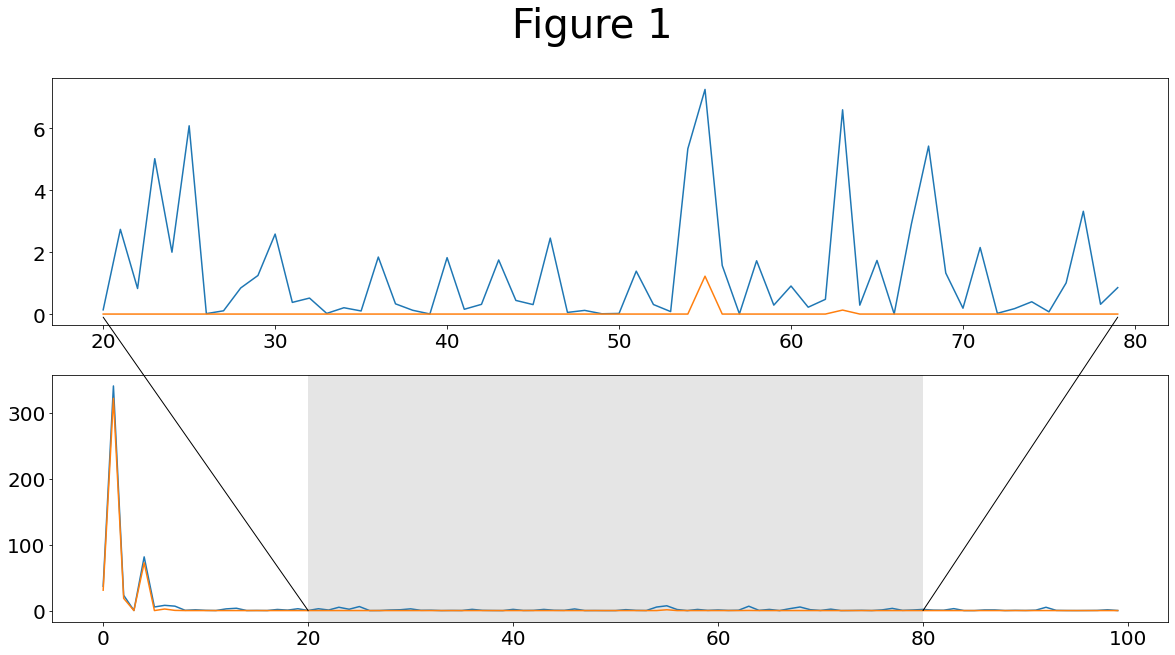

In article

import rpy2
import rpy2.robjects as ro 
from rpy2.robjects.vectors import FloatVector 
from rpy2.robjects.packages import importr

%load_ext rpy2.ipython

%%R
library(GNAR)
library(igraph)

R[write to console]: Loading required package: igraph

R[write to console]: 
Attaching package: ‘igraph’


R[write to console]: The following objects are masked from ‘package:stats’:

    decompose, spectrum


R[write to console]: The following object is masked from ‘package:base’:

    union


R[write to console]: Loading required package: wordcloud

R[write to console]: Loading required package: RColorBrewer

import rpy2

from rpy2.robjects.packages import importr

ebayesthresh = importr('EbayesThresh').ebayesthresh

#import rpy2
#import rpy2.robjects as ro 
from rpy2.robjects.vectors import FloatVector
import rpy2.robjects as robjects
from rpy2.robjects.packages import importr
import rpy2.robjects.numpy2ri as rpyn
GNAR = importr('GNAR') # import GNAR 
#igraph = importr('igraph') # import igraph 
ebayesthresh = importr('EbayesThresh').ebayesthresh

%%R
set.seed(1)
x <- rnorm(1000) + sample(c( runif(25,-7,7), rep(0,975)))

\(X_i\)에서 \(\mu_i\) 추출 가능하는 것을 증명할 예제

%%R
# png("Ebayes_plot1.png", width=1600, height=800)
par(mfrow=c(1,2))
par(cex.axis=2) 
par(cex.lab=2)
plot(x, type='l', xlab="Observed data", ylab="")
plot(ebayesthresh(x, sdev=1),type='l', xlab="Estimate", ylab="")
# dev.off()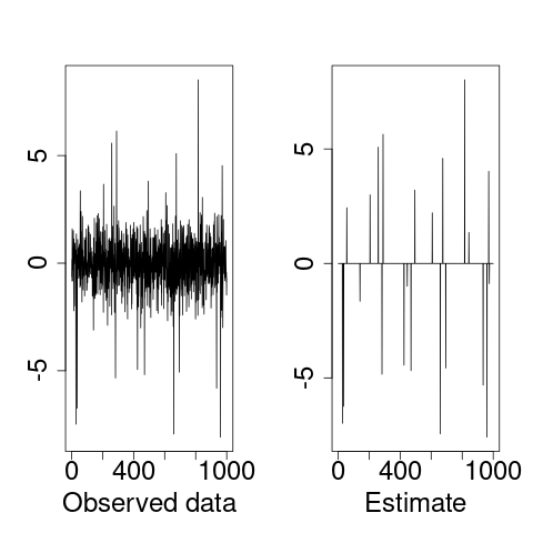

import itstgcn

itstgcn.make_Psi(T)

array([[ 0.07106691, -0.10050378,  0.10050378, ..., -0.10050378,
        -0.10050378,  0.07106691],
       [ 0.10050378, -0.14206225,  0.14184765, ...,  0.14184765,
         0.14206225, -0.10050378],
       [ 0.10050378, -0.14184765,  0.14099032, ..., -0.14099032,
        -0.14184765,  0.10050378],
       ...,
       [ 0.10050378,  0.14184765,  0.14099032, ...,  0.14099032,
        -0.14184765, -0.10050378],
       [ 0.10050378,  0.14206225,  0.14184765, ..., -0.14184765,
         0.14206225,  0.10050378],
       [ 0.07106691,  0.10050378,  0.10050378, ...,  0.10050378,
        -0.10050378, -0.07106691]])

def trim(f):
    f = np.array(f)
    if len(f.shape)==1: f = f.reshape(-1,1)
    T,N = f.shape
    Psi = make_Psi(T)
    fbar = Psi.T @ f # apply dft 
    fbar_threshed = np.stack([ebayesthresh(FloatVector(fbar[:,i])) for i in range(N)],axis=1)
    fhat = Psi @ fbar_threshed # inverse dft 
    return fhat

plt.plot(y)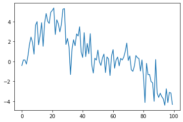

plt.plot(itstgcn.make_Psi(T).T@y)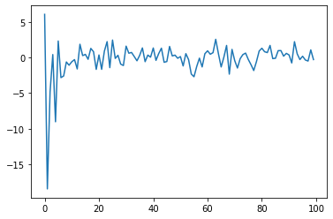

plt.plot(ebayesthresh(FloatVector(itstgcn.make_Psi(T).T@y)))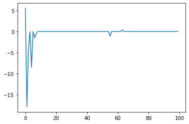

plt.plot(itstgcn.make_Psi(T)@ebayesthresh(FloatVector(itstgcn.make_Psi(T).T@y)))

_T = 1000

_t = np.arange(_T)/_T * 10

_x = 1.5*np.sin(2*_t)+2*np.random.rand(_T)+1.5*np.sin(4*_t)+1.5*np.sin(8*_t)
plt.plot(_x)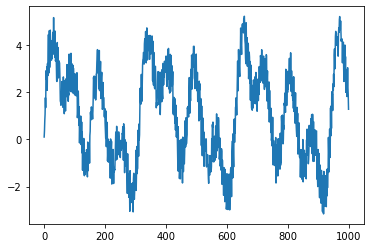

import itstgcn

class Eval_csy:
    def __init__(self,learner,train_dataset):
        self.learner = learner
        # self.learner.model.eval()
        try:self.learner.model.eval()
        except:pass
        self.train_dataset = train_dataset
        self.lags = self.learner.lags
        rslt_tr = self.learner(self.train_dataset) 
        self.X_tr = rslt_tr['X']
        self.y_tr = rslt_tr['y']
        self.f_tr = torch.concat([self.train_dataset[0].x.T,self.y_tr],axis=0).float()
        self.yhat_tr = rslt_tr['yhat']
        self.fhat_tr = torch.concat([self.train_dataset[0].x.T,self.yhat_tr],axis=0).float()

_node_ids = {'node1':0,'node2':1}

_FX1 = np.stack([_x,_x],axis=1).tolist()

_edges1 = torch.tensor([[0,1]]).tolist()

data_dict1 = {'edges':_edges1, 'node_ids':_node_ids, 'FX':_FX1}

data1 = pd.DataFrame({'x':_x,'x1':_x,'xer':_x,'xer1':_x})

loader1 = itstgcn.DatasetLoader(data_dict1)

dataset = loader1.get_dataset(lags=2)

mindex = itstgcn.rand_mindex(dataset,mrate=0.7)
dataset_miss = itstgcn.miss(dataset,mindex,mtype='rand')

dataset_padded = itstgcn.padding(dataset_miss,interpolation_method='linear')

lrnr = itstgcn.StgcnLearner(dataset_padded)

lrnr.learn(filters=16,epoch=10)

10/10

evtor = Eval_csy(lrnr,dataset_padded)

lrnr_2 = itstgcn.ITStgcnLearner(dataset_padded)

lrnr_2.learn(filters=16,epoch=10)

10/10

evtor_2 = Eval_csy(lrnr_2,dataset_padded)

Psi

with plt.style.context('seaborn-white'):
    fig, ax1 = plt.subplots(figsize=(40,15))
    ax1.plot(_x,'k--',label='Observed Data',lw=3)
    ax1.legend(fontsize=40,loc='lower left',facecolor='white', frameon=True)
    ax1.tick_params(axis='y', labelsize=40)
    ax1.tick_params(axis='x', labelsize=40)
    ax1.set_ylim(-6,6)
plt.savefig('Ebayes_fst.pdf', format='pdf')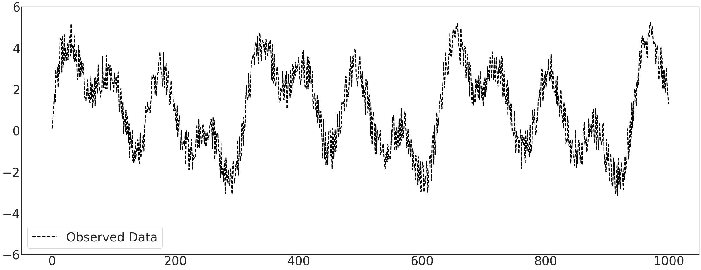

fourier transform

with plt.style.context('seaborn-white'):
    fig, ax1 = plt.subplots(figsize=(40,15))
    # ax1.plot(itstgcn.make_Psi(_T).T@np.array(_x),'-',color='C1',label='Fourier Transform',lw=3)
    ax1.stem(itstgcn.make_Psi(_T).T@np.array(_x),linefmt='C1-',basefmt='k-',label='Fourier Transform')
    ax1.legend(fontsize=40,loc='upper right',facecolor='white', frameon=True)
    ax1.tick_params(axis='y', labelsize=40)
    ax1.tick_params(axis='x', labelsize=40)
plt.savefig('Ebayes_snd.pdf', format='pdf')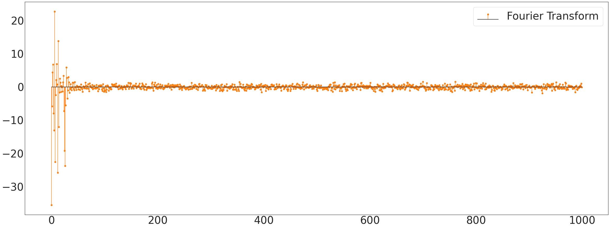

with plt.style.context('seaborn-white'):
    fig, ax1 = plt.subplots(figsize=(40,15))
    # ax1.plot(itstgcn.make_Psi(_T).T@np.array(_x),'-',color='C1',label='Fourier Transform',lw=3)
    ax1.stem((itstgcn.make_Psi(_T).T@np.array(_x))[:100],linefmt='C1-',basefmt='k-',label='Fourier Transform')
    ax1.legend(fontsize=40,loc='upper right',facecolor='white', frameon=True)
    ax1.tick_params(axis='y', labelsize=40)
    ax1.tick_params(axis='x', labelsize=40)
plt.savefig('Ebayes_snd_zin.pdf', format='pdf')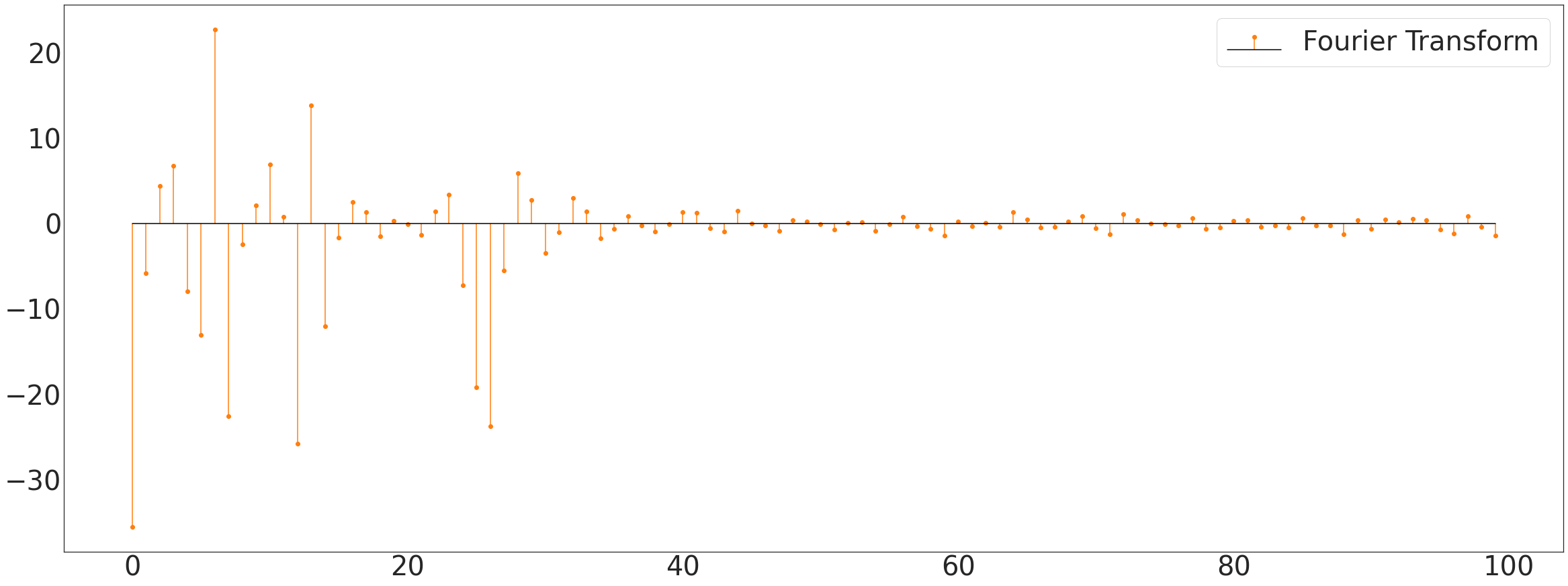

Ebayesthresh/trim

with plt.style.context('seaborn-white'):
    fig, ax1 = plt.subplots(figsize=(40,15))
    # ax1.plot(ebayesthresh(FloatVector(itstgcn.make_Psi(_T).T@np.array(_x))),'-',color='C1',label='EbayesThresh',lw=3)
    ax1.stem(ebayesthresh(FloatVector(itstgcn.make_Psi(_T).T@np.array(_x))),linefmt='C1-',basefmt='k-',label='EbayesThresh')
    ax1.legend(fontsize=40,loc='upper right',facecolor='white', frameon=True)
    ax1.tick_params(axis='y', labelsize=40)
    ax1.tick_params(axis='x', labelsize=40)
plt.savefig('Ebayes_trd.pdf', format='pdf')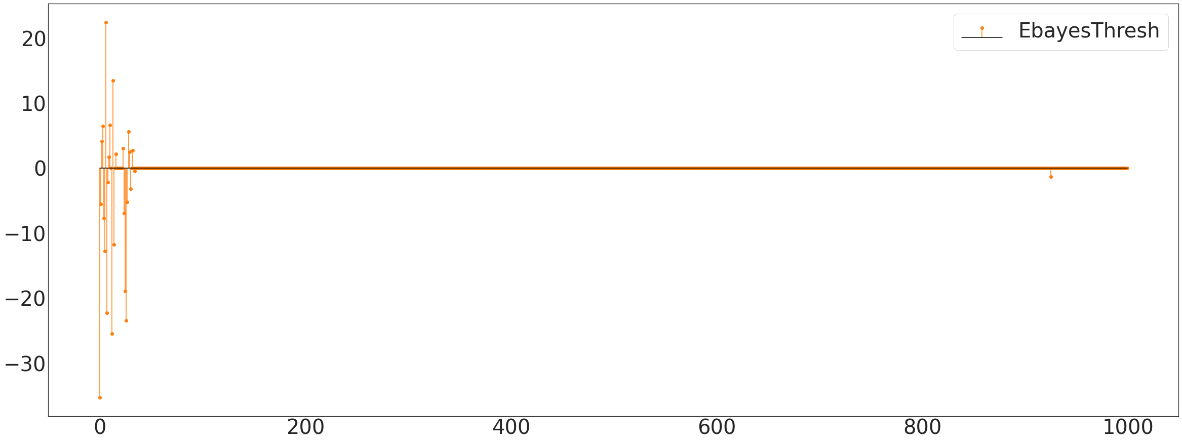

with plt.style.context('seaborn-white'):
    fig, ax1 = plt.subplots(figsize=(40,15))
    # ax1.plot(ebayesthresh(FloatVector(itstgcn.make_Psi(_T).T@np.array(_x))),'-',color='C1',label='EbayesThresh',lw=3)
    ax1.stem((ebayesthresh(FloatVector(itstgcn.make_Psi(_T).T@np.array(_x))))[:100],linefmt='C1-',basefmt='k-',label='EbayesThresh')
    ax1.legend(fontsize=40,loc='upper right',facecolor='white', frameon=True)
    ax1.tick_params(axis='y', labelsize=40)
    ax1.tick_params(axis='x', labelsize=40)
plt.savefig('Ebayes_trd_zout.pdf', format='pdf')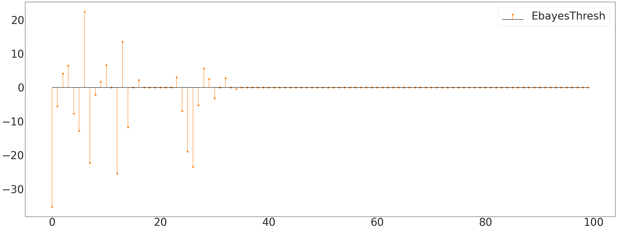

fhat

with plt.style.context('seaborn-white'):
    fig, ax1 = plt.subplots(figsize=(40,15))
    ax1.plot(_x,'k--',label='Observed Data',lw=3,alpha=0.3)
    ax1.plot(itstgcn.make_Psi(_T)@ebayesthresh(FloatVector(itstgcn.make_Psi(_T).T@np.array(_x))),'-',color='C1',label='Inverse Fourier Transform',lw=5)
    ax1.legend(fontsize=40,loc='lower left',facecolor='white', frameon=True)
    ax1.tick_params(axis='y', labelsize=40)
    ax1.tick_params(axis='x', labelsize=40)
    ax1.set_ylim(-6,6)
plt.savefig('Ebayes_fth.pdf', format='pdf')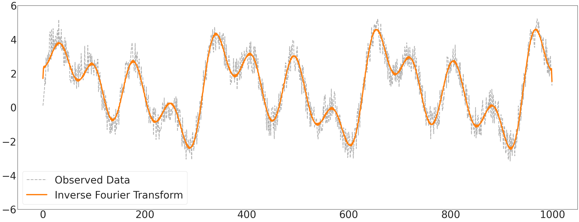

with plt.style.context('seaborn-white'):
    fig, ax1 = plt.subplots(figsize=(40,15))
    # fig.suptitle('Figure 1(node 1)',fontsize=40)
    ax1.plot(data1['x'][:],'-',color='C3',label='Complete Data')
    ax1.legend(fontsize=40,loc='lower left',facecolor='white', frameon=True)
    ax1.tick_params(axis='y', labelsize=40)
    ax1.tick_params(axis='x', labelsize=40)
# plt.savefig('node1_fst.png')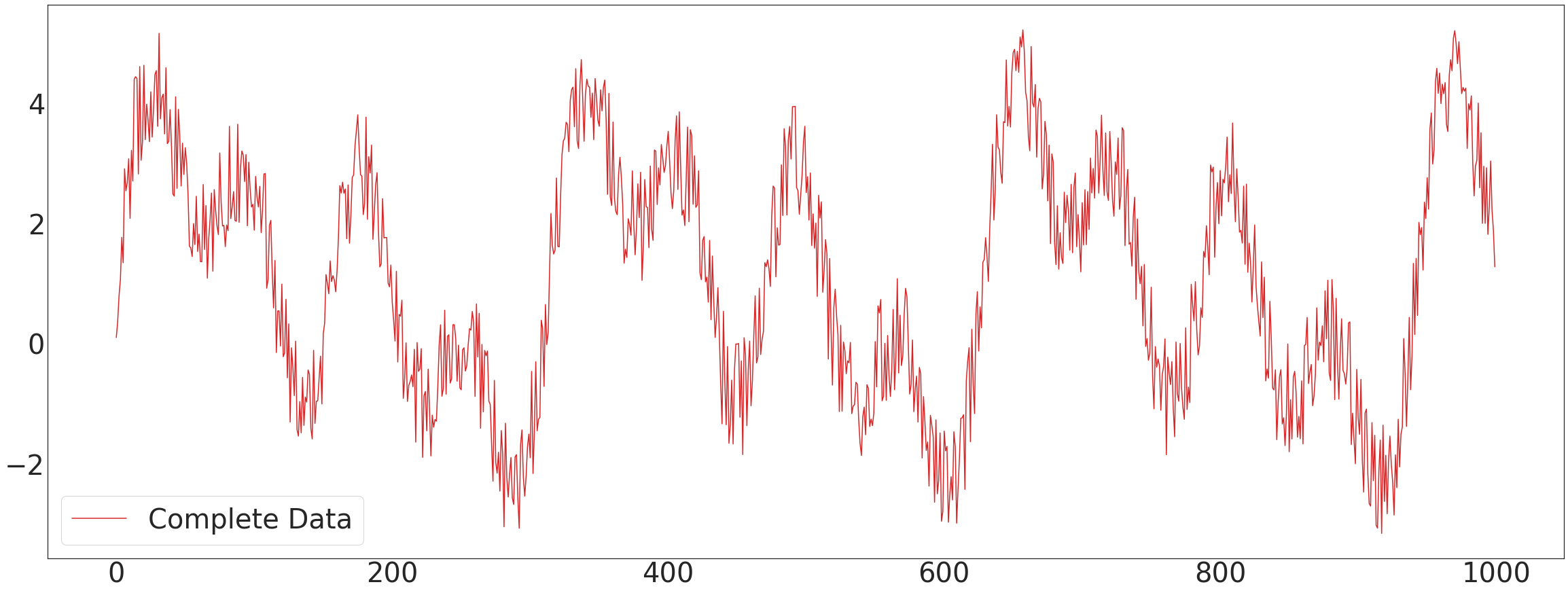

with plt.style.context('seaborn-white'):
    fig, ax2 = plt.subplots(figsize=(40,15))
    # fig.suptitle('Figure 1(node 1)',fontsize=40)
    ax2.plot(data1['x'][:],'--',color='C5',alpha=0.5,label='Complete Data')
    ax2.plot(torch.cat([torch.tensor(data1['x'][:4]),torch.tensor(dataset_miss.targets).reshape(-1,2)[:,0]],dim=0),'--o',color='C3',label='Observed Data',markersize=15)
    ax2.legend(fontsize=40,loc='lower left',facecolor='white', frameon=True)
    ax2.tick_params(axis='y', labelsize=40)
    ax2.tick_params(axis='x', labelsize=40)
# plt.savefig('node1_snd.png')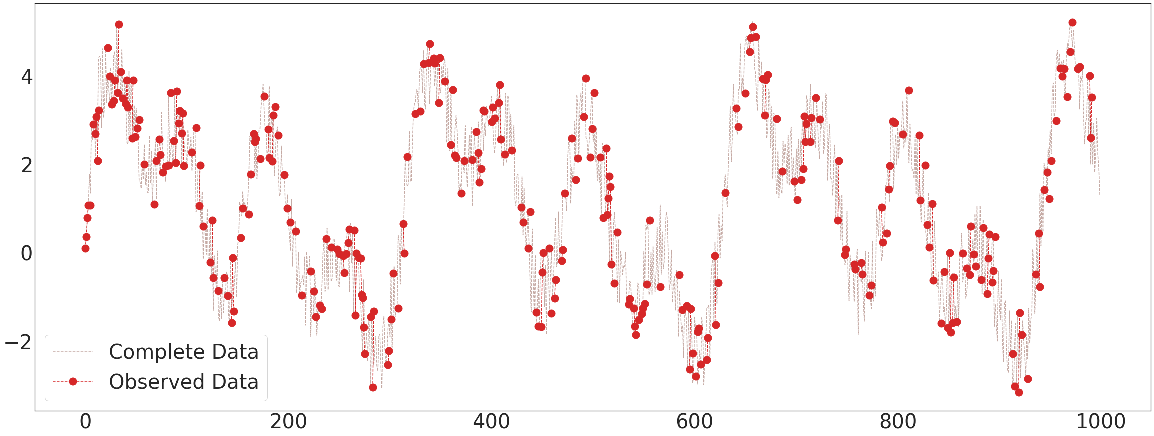

with plt.style.context('seaborn-white'):
    fig, ax3 = plt.subplots(figsize=(40,15))
    # fig.suptitle('Figure 1(node 1)',fontsize=40)    
    ax3.plot(data1['x'][:],'--',color='C5',alpha=0.5,label='Complete Data')
    ax3.plot(evtor_2.f_tr[:,0],'--o',color='C3',alpha=0.8,label='Interpolarion')
    ax3.legend(fontsize=40,loc='lower left',facecolor='white', frameon=True)
    ax3.tick_params(axis='y', labelsize=40)
    ax3.tick_params(axis='x', labelsize=40)
# plt.savefig('node1_3rd.png')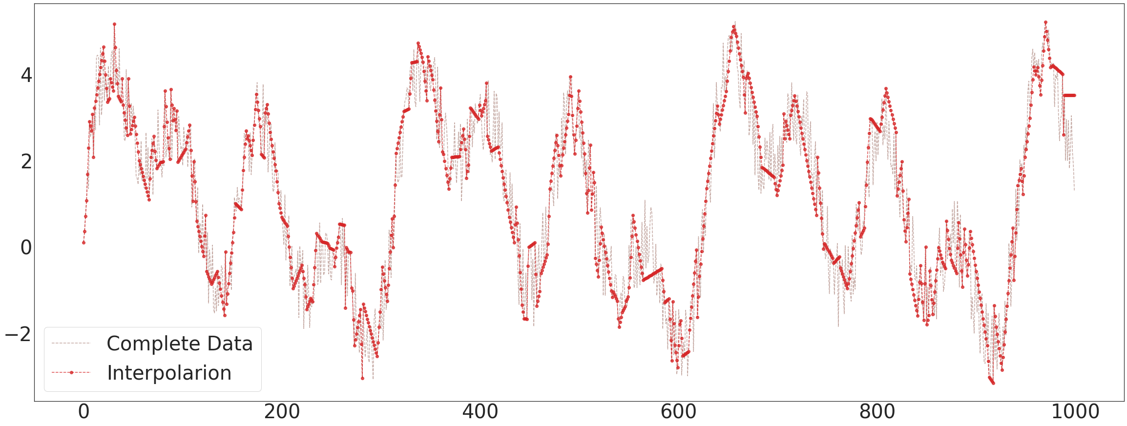

with plt.style.context('seaborn-white'):
    fig, ax4 = plt.subplots(figsize=(40,15))
    # fig.suptitle('Figure 1(node 1)',fontsize=40)
    ax4.plot(data1['x'][:],'--',color='C5',alpha=0.5,label='Complete Data')
    ax4.plot(evtor.fhat_tr[:,0],color='brown',lw=3,label='STGCN')
    ax4.plot(evtor_2.fhat_tr[:,0],color='blue',lw=3,label='ITSTGCN')
    # ax4.plot(138, -1.2, 'o', markersize=230, markerfacecolor='none', markeredgecolor='red',markeredgewidth=3)
    # ax4.plot(220, -1.5, 'o', markersize=200, markerfacecolor='none', markeredgecolor='red',markeredgewidth=3)
    # ax4.plot(290, -1.2, 'o', markersize=310, markerfacecolor='none', markeredgecolor='red',markeredgewidth=3)
    # ax4.plot(455, -0.9, 'o', markersize=280, markerfacecolor='none', markeredgecolor='red',markeredgewidth=3)
    ax4.legend(fontsize=40,loc='lower left',facecolor='white', frameon=True)
    ax4.tick_params(axis='y', labelsize=40)
    ax4.tick_params(axis='x', labelsize=40)
# plt.savefig('node1_4th_1.png')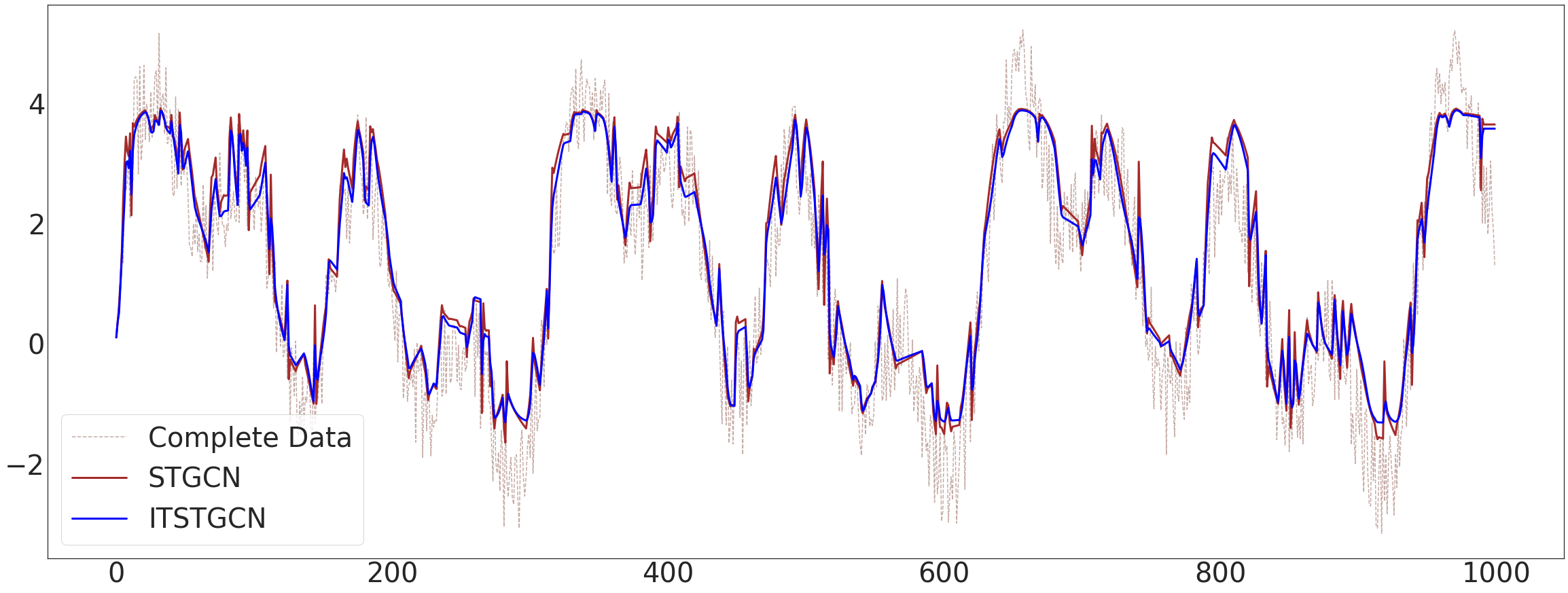

For Paper

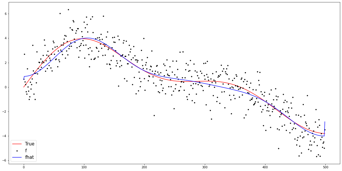
T = 500

t = np.arange(T)/T * 10

y_true = 3*np.sin(0.5*t) + 1.2*np.sin(1.0*t) + 0.5*np.sin(1.2*t)

y = y_true + np.random.normal(size=T)

plt.figure(figsize=(20,10))
plt.plot(t,y_true,color='red',label = 'true')
plt.plot(t,y,'.',color='black',label = 'f')
plt.legend(fontsize=15,loc='lower left',facecolor='white', frameon=True)
# plt.savefig('1.png')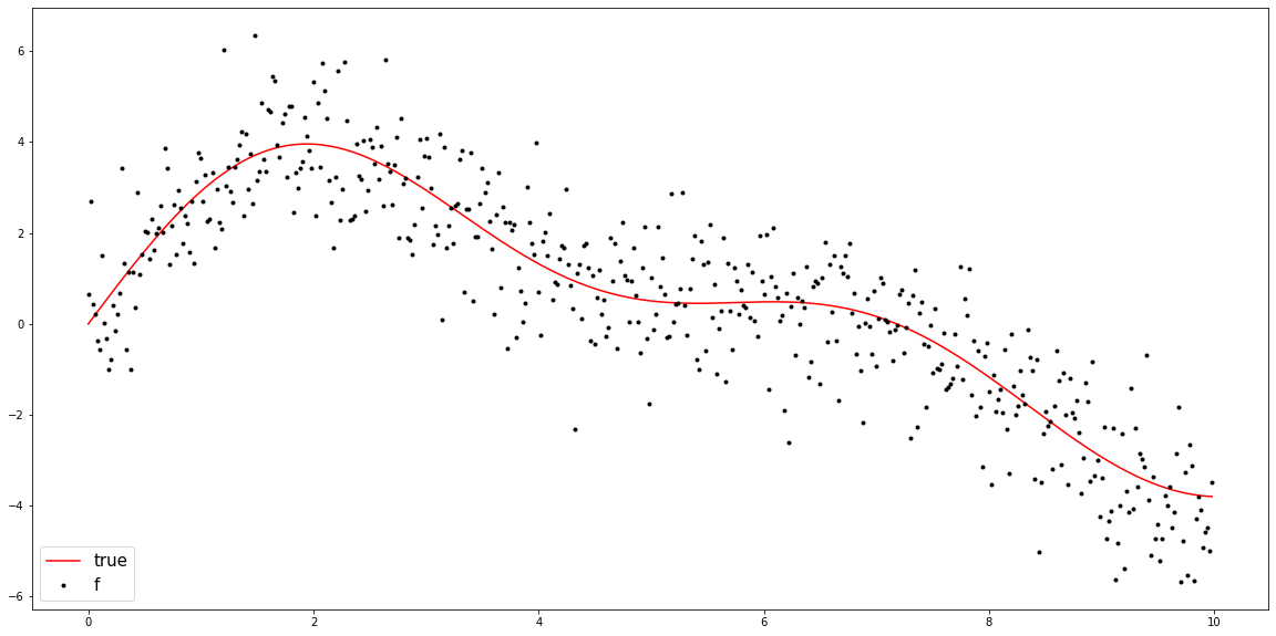

f = np.array(y)
if len(f.shape)==1: f = f.reshape(-1,1)
T,N = f.shape
Psi = make_Psi(T)
fbar = Psi.T @ f # apply dft

fbar_threshed = np.stack([ebayesthresh(FloatVector(fbar[:,i])) for i in range(N)],axis=1)

plt.figure(figsize=(20,10))
plt.plot(fbar**2,color='black')
# plt.savefig('1.png')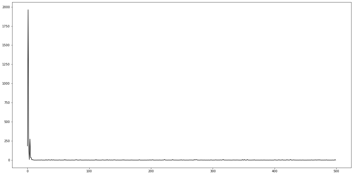

plt.figure(figsize=(20,10))
plt.plot(fbar_threshed**2,color='blue')
# plt.savefig('2.png')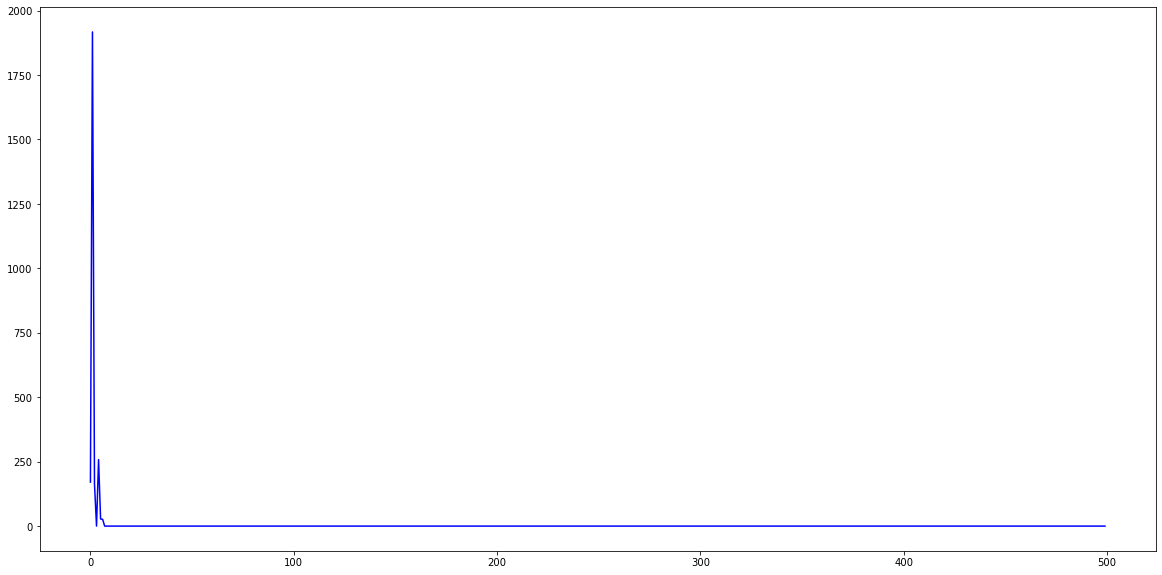

plt.figure(figsize = (20,10))
ax = plt.subplot(1, 1, 1)
ax.plot(range(0,500),(fbar**2),color='black')
ax.plot((fbar_threshed**2),color='blue')
axins = inset_axes(ax, 8, 3, loc = 1, bbox_to_anchor=(0.8, 0.8),
                   bbox_transform = ax.figure.transFigure)
axins.plot(range(100, 200),(fbar**2)[100:200],color='black')
axins.plot(range(100, 200),(fbar_threshed**2)[100:200],color='blue') 
axins.set_xlim(100, 200)
axins.set_ylim(-0.1, 7)
mark_inset(ax, axins, loc1=4, loc2=3, fc="none", ec = "0.01")
ax.tick_params(axis='y', labelsize=20)
ax.tick_params(axis='x', labelsize=20)
axins.tick_params(axis='y', labelsize=15)
axins.tick_params(axis='x', labelsize=15)
# plt.savefig('3.png')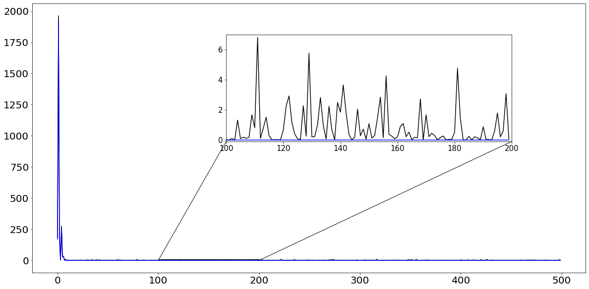

plt.figure(figsize=(20,10))
plt.plot((fbar_threshed**2),color='blue')
# plt.savefig('4.png')

fbar_hat = Psi @ fbar_threshed # apply dft

plt.figure(figsize=(20,10))
plt.plot(y_true,'r',label = 'True')
plt.plot(y,'k.',label='f')
plt.plot(fbar_hat,color='blue',label = 'fhat')
plt.legend(fontsize=15,loc='lower left',facecolor='white', frameon=True)
# plt.savefig('5.png')